Atakua's Diary

Raster to vector conversion for land cover

The whole premise of the land cover import for Sweden [1] bases on the idea to take the raster map of land cover and to covert it into the OSM format. This results in new map features that are essentially closed (multi)polygons and tags. These new features are then integrated into the existing database with old features during the conflation step.

This post is about the first steps of this process, everything around the vectorization of raster.

Data flow overview

It is hard to describe all the programmatic and manual actions needed to convert the input data. A lot of it is described in the OSM wiki page [1]. The best way to learn the details is to look into the source code of scripts written to achieve the goal. However, the general data processing flow will definitely contain most of the following phases, and maybe something more. The order of certain steps, especially filtering phases, can be different. Coordinate system transformations are only needed if the input data is not in the WGS 84 format used by the OSM database. It can also be done later in the process.

Change coordinate system of data
Filter the input raster file to remove small “noise”
Remap input raster to reduce number of pixel classes
Mask the input raster with a mask raster generated from existing OSM data
Split te single raster file into smaller chunks i.e. tiles
Vectorize the raster data into vector data
Assign OSM tags to vector features, drop uninteresting features
Smooth the features to hide the rasterization artifacts
Simplify the features to keep size of data in check
Do automatic conflation steps that take both new and old vector data into the account. Examples: cut roads, snap nodes, delete insignificant features etc.
Do manual conflation steps that could not be automated.

Raster masking approach

To recap on relations between raster and vector layers of new and existing data to be conflated with each other.

It proved difficult to automatically or even manually make sure that land use (multi)polygons from existing OSM-data and new data to be imported do not conflict with each other when they both are represented as vector outlines. Even more complex question is how to decide what to do with two conflicting ways. Should one delete one of them? Replace one with another? Merge them? Create a common border between them?

A simpler approach was developed to address conflicts at the stage when import data can be easily masked, i.e. when it is represented by raster pixels. The idea behind this approach that we can generate a second raster image of identical size and resolution for the country. The source for this raster mask image is existing OSM land cover information. For example, a vector way for already mapped forest will be turned into a group of non-zero pixels. The vectorizing software then uses this mask to prevent new vector ways to be created from the import data raster. It would look as if no data for those areas is available. As a result, vectors generated from masked raster never enter “forbidden” areas where previously mapped OSM-data is known to be present.

By restricting new data to be created only for not yet mapped areas we reduce the problem of finding intersections between multipolygons to the problem of aligning borders between new and old polygons.

As import data is masked at the very first stage when it is in raster form, it is expected that areas “touching” (sharing common border) with pre-mapped land cover data will require careful examination and merging of individual way borders. All cases of overlapping of identical land uses should be fixed.

Issues with tagging

A major issue that everyone is wary of is that new features generated from the import data will be incorrectly tagged. The issue here is that the OSM tagging approach does not stimulate using fixed predetermined number of data classes for land cover, meanwhile the majority of raster sources by definition provide a limited number of pixel values and associated landuse classes. Mapping the former to the latter is considered by some to be the most unreliable task.

Sure, there were situations when a misclassification of a feature was found during cross-inspection of new data, old data and aerial imagery. But they were really rare compared to numerous other problems to deal with. The most common (but still rare) situation of this class was wrong marking of “bushes” under a power line as “forest”.

The real problem was in the need to adjust the tag correspondence map from input raster values to resulting OSM tags. That is, in different regions of the country the same pixel value might correspond to different OSM tags.

The most problematic class of land cover to tag correctly turned out to be “grass”. The same original raster pixel value may correspond to different concepts in OSM, ranging from a golf course, through cultivated grass to wild or cultivated meadow and even heathland. Because of that, manual inspection of all areas tagged as “grass” was constantly needed.

Excessively detailed ways

Often more nodes that a human would place are used on a way. Original data may have a node every 10 meters, additionally using Chaiken [2] filter to smooth 90-degrees in vector data can create as many nodes. See an example:

Excessive details

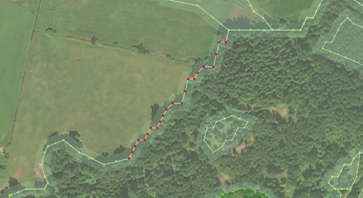
A manual solution is to delete undesired nodes, and/or use Simplify way [3] tool to do so.

An automatic solution would be to apply Douglas-Peucker filter to ways of the import file. The issue is to find the best threshold values for the simplification algorithm. Excessively aggressive automatic removal of nodes leads to losing important details of certain polygons. Typically it can be expected that up to 50% of import data set nodes can be removed without losing much in quality of details.

It seems that an extra pass with v.generalize douglas threshold = 0.00005 does a good enough job without chewing too much of details. It does, however, chew some important details, especially of bigger polygons (such as those at a tile border), and also fails to clean up segments that are shared between several ways. Because of the last issue, manual phases of detecting and smoothing remaining angles with 90-degrees and close pairs of nodes that are strictly horisontal or vertical were necessary to implement to clean up suspicious geometry patterns left after vectorization, smoothing and simplifying phases.

General notes on manually vs machine traced polygons

Pros of machine traced land cover.

Consistency in making decisions at tracing. Humans’ decisions during the tracing are largely affected by a lot of random factors including the level of concentration, tiredness, smoothness of mouse/pointer operation etc. A person may skip the whole section or oversimplify it because he feels so right now. Another human or even the same one but at a different time of the day would have produced a completely different result. A computer algorithm is consistent and uniform in its both good and bad tracing decisions. Given that we can improve on the algorithms, the ratio of good to bad machine tracing can be monotonically improved.
Computers won’t get tired until it is done with tracing. Time needed to find complete borders of a forest section is often underestimated as it just goes on and on. The started tracing line just won’t return back to the beginning even if it may return temptingly close to it several times. A human will decide sooner or later to (literally) draw a line and end the current polygon prematurely even if it is clear that more can be included into it. The next part will have to be traced separately as a new polygon. A computer, on the other hand, is fast enough to trace everything under reasonable time. It won’t stop until it is done. Often the only limit for it are physical limits of current map tile, not the length or complexity of the resulting polygon.

Pros of human traced results.

“Important” features get traced first. It is hard to algorithmically define what is important at current map position as this largely depends on the context. A common approach for a computer is to process everything at hand, as it can afford it because it is so fast. Humans can “feel” the context and use it efficiently to prioritize things. For example, one typically starts from working on bigger features that are close to populated areas and which are likely to be looked in the end.
Tag choice is more consistent with reality. It is well known problem in remote land cover sensing that no 100% correct matching can be achieved. Again, this is in part because not everything can be tagged with a limited number of classes and corresponding tag combinations. Humans tend to be more conservative in this regard and provide more reliable results. If a person cannot tell from looking at the image what sort of land cover should be given to a polygon, he is likely to skip it altogether or at least express his doubts in a comment to the tag set. The machine is rarely tasked with recording its confidence level for the chosen tags.
Humans tend to choose vector resolution (distance between nodes) dynamically based on current context. For example, a forest around a long straight highway tends to be mapped with few nodes along that road. More nodes are needed when a forest border is more “open” and does not contact anything else. Machine algorithms are currently not taking the context into account and basically use a fixed resolution coming from the underlying raster image. Different smoothing or simplification algorithms do not change this much as they only take into account the current curve itself, not adjacent data. Because of that both situations are possible with machine processed data: a) a lot of extra nodes along a straight line that could have been mapped with just a few of them; b) lost important nodes where a line takes a sudden turn.

The same applies to making decisions of which features to keep. It was common to get many small patches of grass along highways that face large forests from machine-traced data. A human would have ignored these patches and drew a single line between a forest and a highway.

Common issues:

It is impossible to “naturally” determine where one should stop tracing a polygon, round it up and go for the next one. A machine traces it until it has some data left to trace, e.g. until it naturally closes the current polygon or reaches an artificial border of current raster area. A human traces until he gets tired, then he simply draws a straight line to the beginning and calls it fine. Both approaches have their problems. Humans tend to round up in a way that simplifies future additions by e.g. closing polygons through areas that are of less importance and where no future details are expected to be added. A computer may finish its work right in the middle of tightly populated area, thus creating a lot of complications for someone who wants to complete mapping of remaining area.