Land cover conflation. Practical issues

This is the third part of summarizing my experience with conflation of land cover data for Sweden. More examples of practical problems and ways to address them follow.

The same or similar problems may or may not arise during other imports of closed (multi)polygons in the future, so tips and tricks to save time will become handy. Note that some points from the previous part may be repeated here, but with more thoughts or ideas on how to address them.

Why bother with land cover import

The general idea of importing any data into OSM is to save time on doing the same by hand.

Classic data sources for the OSM contents are:

1. Local or public knowledge. This is mostly useful for points of interest, provided one knows an exact position of the point. For needs of land cover, local reconnaissance is critical for establishing secondary details of actual surface. E.g., for a swamp, what type of swamp, for a forest, what species of trees, with what height/diameter and of what age. There are remote sensing methods, however, that allow obtaining some of this information in some cases without visiting the actual place.

2. GPX traces submitted by users. These are very useful for mapping certain linear objects such as roads. This is natural as people tend to move along the roads. But people do many other things for which a map would be helpful, but obtaining accurate linear traces is problematic. For closed map features, such as building outlines, usefulness of GPX traces becomes limited as people rarely use to circle around each and every house. Besides, the baseline GPS resolution of several meters (without a lengthy precision improvement procedure) is often not enough to make out where actual corners of a building are. To go around a swamp in a remote location to get its outline is rarely doable in reasonable time.

3. Aerial and satellite imagery. Provided the pictures are up-to-date and do not have an unknown offset relative to reality (which GPX traces can help establish and correct as a cross-referencing source), the imagery allows to trace basically everything that is visible on the earth surface. The problem is that amount of data this source gives is overwhelming. The only universally accepted way to convert it to vector is manual tracing, which is a not very efficient way to process data given that it is done on a computer that is capable of billions operations per second.

The benefits of a data import is that instead of tracing aerial images and/or GPX traces, we simply get “ready” data.

This data is also very likely to contain “noise” — any sorts of artifacts, wrong points, extra useless data etc. Balancing the value of new data against amount of new issues it brings into the database should always be held in check. This is a classical “signal to noise ratio” problem. To determine what kind and level of noise is acceptable is essential. Whether it is comparatively easy to ignore or manually remove the noise present in data generated by the scripts determines when it is worth trying importing data and fixing it at the same time. It may turn out that it is faster to simply trace everything manually or to get the data from another source.

An important aspect of land cover features is their inherent redundancy and inexactness of their geometry. You can often delete a node of a polygon denoting a forest or move it slightly without significantly affecting the perceived accuracy of how the its reflects the reality. This opens possibilities for optimizations such as adjusting common boundaries of features.

Complexity metric for data batches

It turned out to be useful to have a rough estimation of how hard a particular tile would turn out to integrate by calculating a complexity metric over it.

Intuition says that the more input data there is in the new data layer or in the old data layer, the harder it would be to make sure that they are nicely aligned. But what is the best mathematical expression to quantify this idea?

Originally, a total sum of number of new and old ways was used as a complexity metric.

It kind of made sense because a lot of conflation work is done to align common shared borders between new and old ways. It did not matter how many nodes were there, and relations typically did not stand in the way of doing it as mostly outer ways were important.

Later in the process is was decided that even a simpler metric is more representative of what needs to be done to integrate a tile. Namely, number of old ways proved to be proportional to how much time will be spent on aligning new ways to them.

Further refinements to the metric is of course possible. Seeing the complexity number along a list of not yet processed tiles allowed to understand which tile should be opened next to make sure it will be possible to process it under a limited span of time.

Excluded and missing features

The import raster file stored information for the whole country area and a wide assortment of land use classes, including those common for wilderness, residential, water areas, as long as rail- and car roads.

Information about roads was clearly least useful. As an assortment of pixels, there was no guarantee for proper connectivity for roads, which is the main property to extract and preserve in a vector map that should allow routing.

Residential areas were also excluded as the raster resolution of 10×10 meters did not allow to reconstruct actual footprints of individual buildings. There is however an idea to use this information to partially map remote isolated dwellings, if not as polygons then at least as nodes building=yes.

It was finally decided not to import water bodies, such as lakes, swamps and rivers but to focus on forests, farmland and grass. This is despite the fact that information about water bodies was in fact extractable from the import raster.

The motivation for the decision not to use them was based on the following premises.

1. Water bodies would be already well represented in the OSM. This turned out not to be true for many parts of the country. As a result, now the map has “white holes” where not yet mapped lakes should be in reality.

2. Decision to import land cover for islands and islets. This was in conflict with the developed approach of using a separate mask raster layer that did not treat water areas as masked. Including mapped lakes into the mask layer would have masked islets.

Ideas on how to import water bodies

As we can see now, the OSM map would benefit from a careful import of missing lakes as well.

It should be possible to import water bodies in a separate process from the same input raster. The import data processing scripts will have to be adjusted in many places to take into account different status of lakes. In particular:

1. The mask layer should include “landuse=water” to prevent creation of overlapping water bodies. Ocean/sea around the coastline have to receive the same treatment to avoid mapping water inside the ocean. However, areas outside the coastline borders are likely to already be marked as “no data” in the source raster image.

2. To prevent “slivers” of water in the shore area (similar to noise around already mapped forests), limitations of how “oblong” new water features can become should be set in the scripts. This means that wider rivers will most likely be excluded from the end result.

3. The naive tiled approach with static extent positions would lead to cutting of new lakes into several adjacent pieces. To avoid this, tiles should dynamically be resized to implement the “all or nothing” approach for water bodies. The idea is that, while a forest can be split into several adjacent pieces that can be individually mapped, a feature for a lake is typically added as a whole area. It may be represented as a multipolygon with multiple shorter outer boundaries if needed, but the result should not look like two separate water bodies with a common border along a tile edge. At least this is not how one usually maps lakes in the OSM. If nothing else, larger tile sizes would decrease amount of cases of clipped water bodies. And in remaining cases two or more pieces should be merged into a single polygon, not just aligned to have a single common border.

4. Making sure the border between land and water is unified will be a tough problem to automatically solve, given the amount of land cover data already imported.

Boundaries between individual tiles

Tiles as rectangular extents of data of the same size and adjacent to each other are one of simplest methods to split huge geodata into smaller chunks that are easier to work on individually. However, the transition from one tile to adjacent ones should still be smooth in the resulting vector data. The most apparent problem that comes to mind is positive or negative gaps between features lying close to common borders of adjacent tiles.

During this import the following problems with tile boundaries were observed.

1. A bug in a tile splitting algorithm caused adjacent tiles to overlap significantly (up to several hundreds meters). This defect in resulting vector data was very cumbersome to manually fix, especially when at least one of the overlapping tiles had already been uploaded to the database. Careful ordering of coordinate system conversions allowed to avoid this issue and generate further tiles with much better mutual alignment.

2. Smoothing algorithms tended to move nodes including tile border nodes. Nodes at four corner positions of the rectangle suffered most often — they were “eaten” by the Douglas-Peucker algorithm and required manual restoration at the editing phase. In general, the edges of the tile is the area where “sharp” corners in features should be allowed. But curve simplification algorithms tend to replace them with more gradual transitions.

3. Rounding error accumulated at different data processing stages caused that boundary nodes were moved by a small fraction of a degree. This regularly caused a tiny (around 1e-4 degrees) but noticeable (bigger than 1e-7 resolution that OSM uses internally) overshoot or undershoot against nearby parallel tile borders. To compensate for it, a separate data processing stage was written to determine which nodes are likely to be “boundary” in the tile. It them made sure that their respective longitude or latitude values would precisely lie on the tile border. For example, all nodes with longitude 45.099998 would be moved to 45.1. This improved the situation somewhat, often making at least some of nodes on two adjacent tile borders to receive identical coordinates and thus allowing for automated merging of feature nodes at such cases.

1. Small features split over into two separate tiles typically did not align well when sewn back together.

It required a manual movement of nodes in both lat/lon directions to restore the original shape. Ignoring a minor misalignment for a small remote natural feature was often fine (who cares if this tiny swamp looks cut?), but when the cut line went through a residential area, one would certainly want to restore the original shape.

Despite some implemented measures for automatic tile border merging, a lot of manual adjustment work was required in many cases. This activity was one of limiting factors for data import speed. Clearly there is a room for improvement for future imports. I see two possible directions.

1. Improving algorithms for feature reconstruction after they were split and parts were individually traced.
2. Improving the tile borders selection algorithms. Instead of just blindly cutting everything without any regard to what lies under the knife, tiles can be made to follow more natural shapes of the data in hand, e.g. preferring cutting through water areas and avoiding separating data in residential areas. Such tiles will be of different size and not necessarily rectangular in shape.

Even using bigger tiles reduces number of cuts in the original data and amount of follow-up sewing of tiles. E.g. instead of cutting a country into small tiles one can split it into bigger counties. However, with a chunk size growing other problems of scale become more prominent. So finding a balance here is critical.

Single and double borders between features

Often it is desirable that two adjacent features have a single border line shared with each other, not two loosely curves intersecting back and forth.

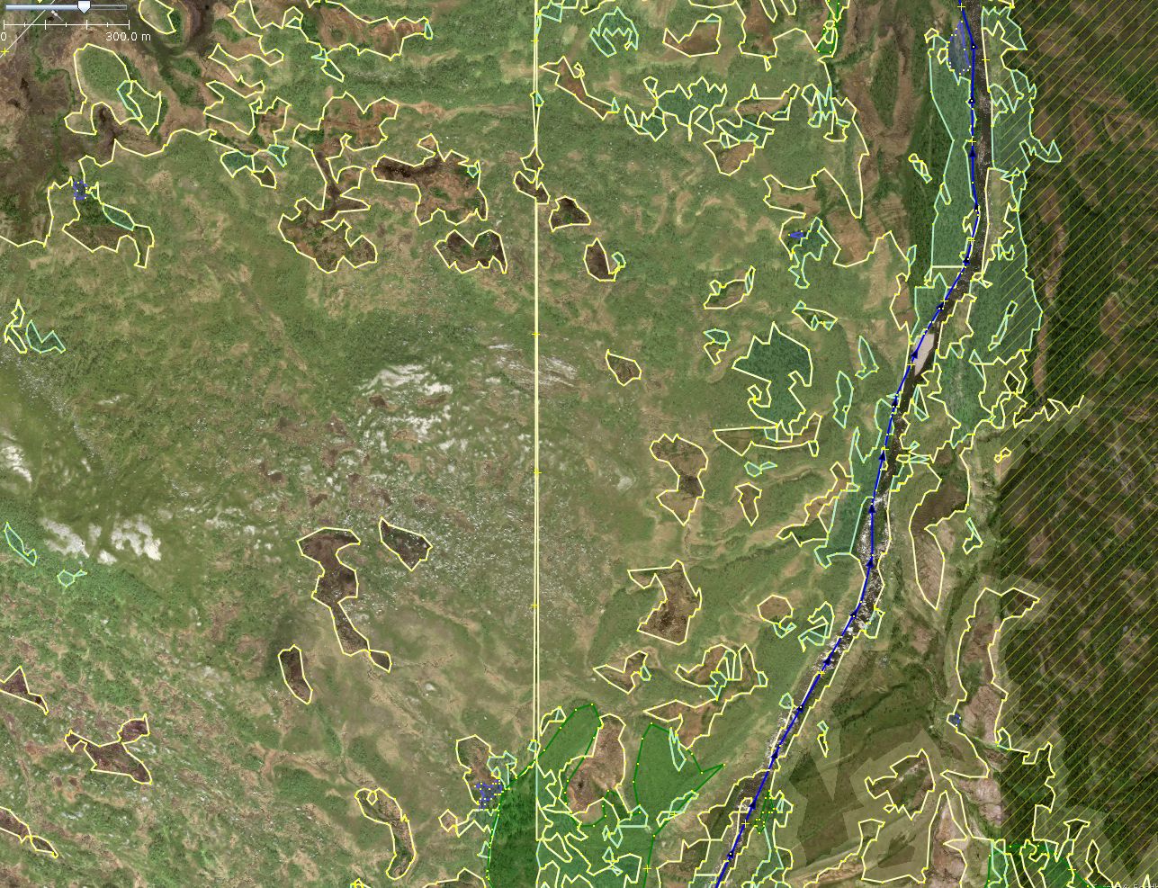
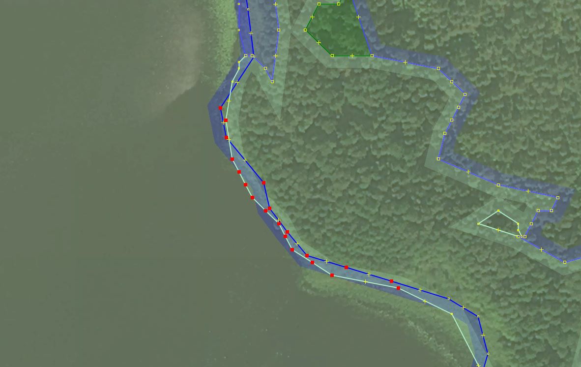
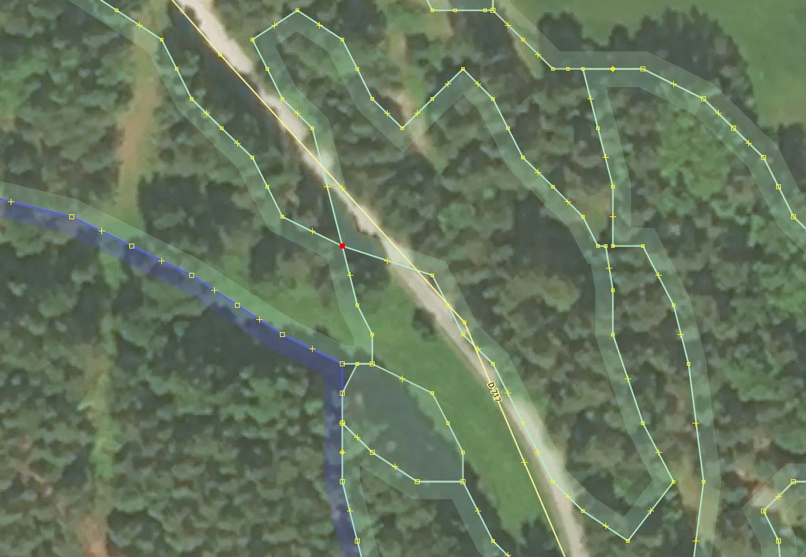
A single border between forest and lake can be seen along the south coast of the lake, while the north coast has a CORINE import forest polygon with its own border running along the lake border.

In my opinion, having a single common border between land cover features is the best. It is more compact to store and less visually complex. It does not correspond to reality in the regard that there is often no sharp border between two natural features.

Double separate borders kind of reflect this fact that one border is not necessarily defined by another feature. However, there are always unanswered questions about what is in between these two features. What is going on in the thin sliver of no data squeezed in between two borders? Is the distance between two features wide enough to reflect the transitional area? What if one of borders is more detailed than another — is it just an artifact or faithful reflection of reality?

Both types of borders are the main problem during the conflation. To maintain a single border between new and old features means to modify existing borders. To create double borders one has to deal with the fact that multiple overshoots and undershoots are about to happen, and as a result these borders will “interlace” with multiple intersections along their common part.

Current semi-automatic methods to maintain the single border, besides manually editing all individual nodes, are:

• Snapping nodes to nearby lines.
• Breaking polygons at mutual intersections and removing smaller overlapping chunks as noise.

The plugin SnapNewNodes [4] was made with idea of helping with the snapping process. It does help, but has annoying bugs making it less reliable. SnapNewNodes should be made more reliable in the result, and report cases when it cannot unambiguously snap everything.

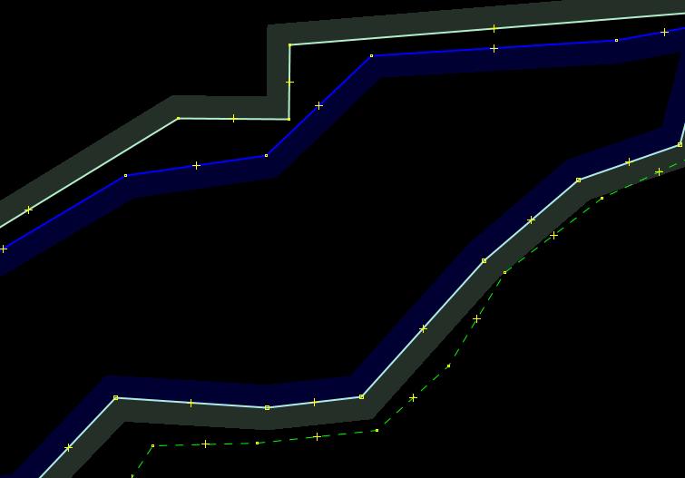
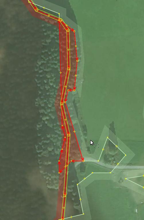
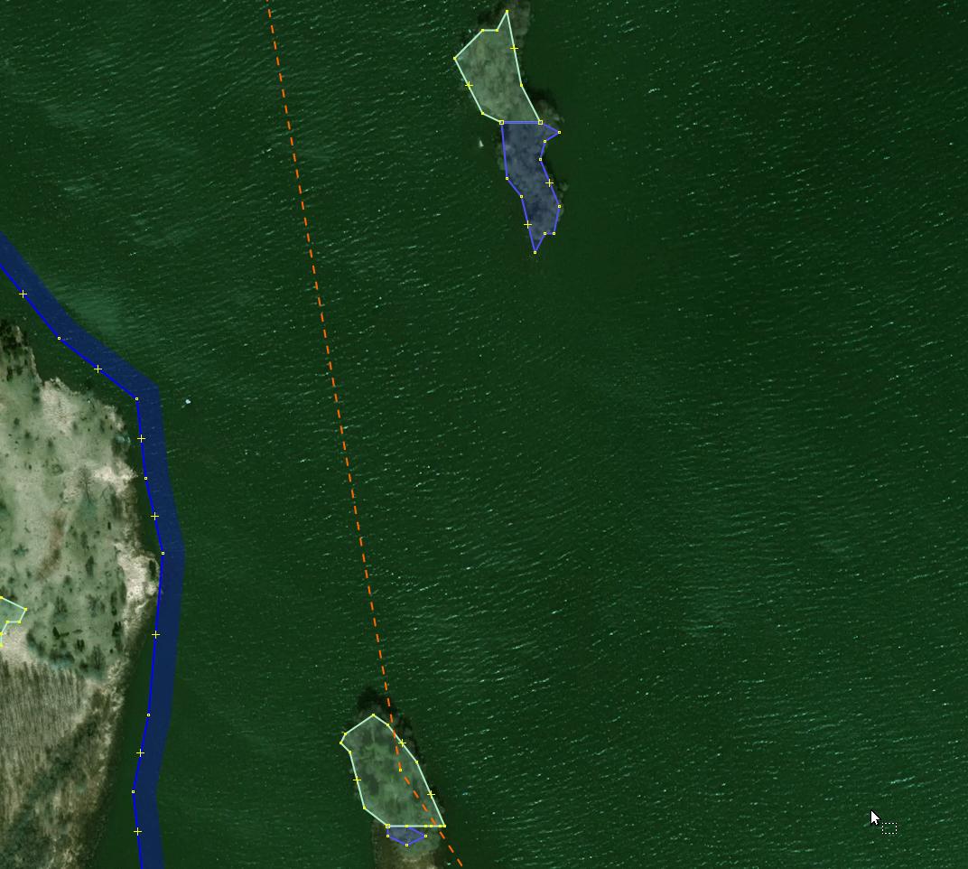
In the import process, the main source of double borders were existing shore lines of lakes and new imported forests, swamps etc.

An interesting case when existing islets without land cover received it from the import data:

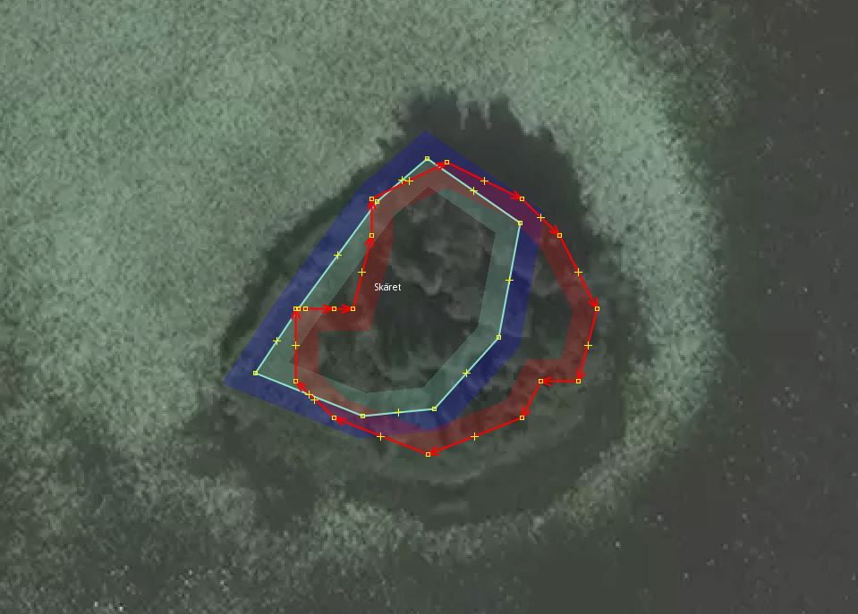
Often the previously mapped water border was of lower quality/resolution than newly added forest bordering with it. But as often both new and old borders were equally accurate.

Still, this resulted in forest partially “sinking” into water and partially remaining on an islet.

Manual solutions include:

• Replacing geometry for small islets to better reflect land cover and aerial images.
• Deleting, merging and snapping nodes of new and old ways to make sure land cover stays within the designated borders. ContourMerge [3] is also useful to speed things up.

Roads partially inside a forest, partially outside it

It has to be manually cut through with two “split way” actions:

This is very laborious and not always possible in cases of multiple inner/outer ways of a multipolygon as they are not considered as a single closed polygon that could be cut through:

Something has to be improved in order to speed up processing of such cases.

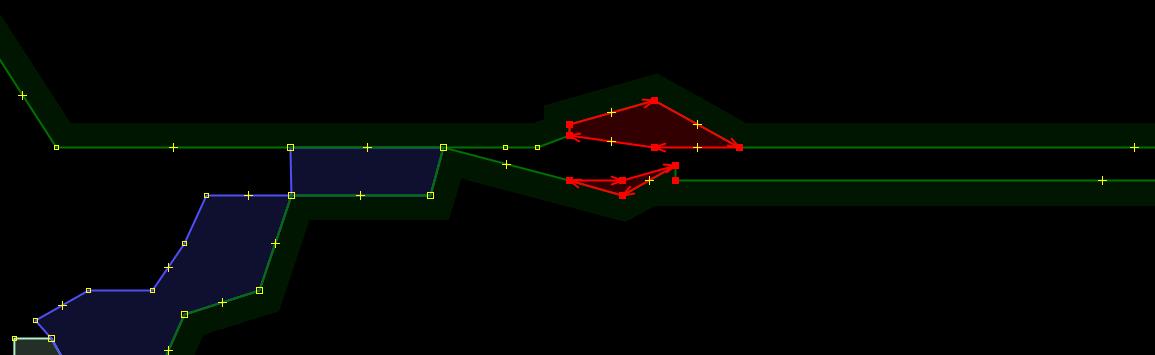
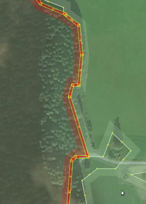
Occasional isthmuses between two land use areas separated by road

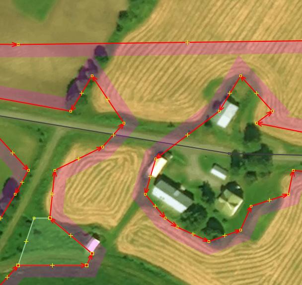
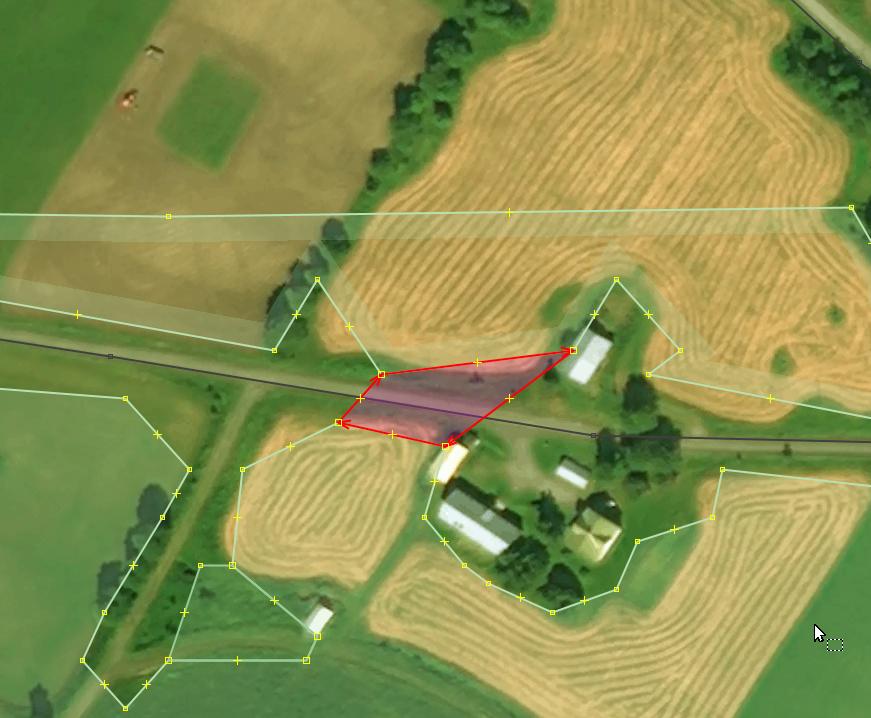
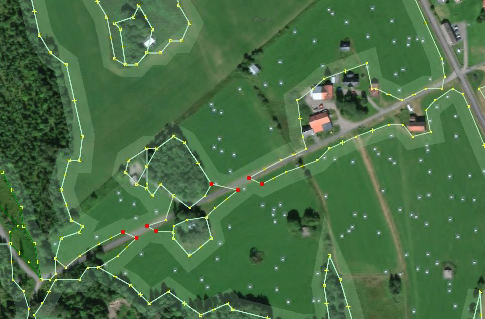
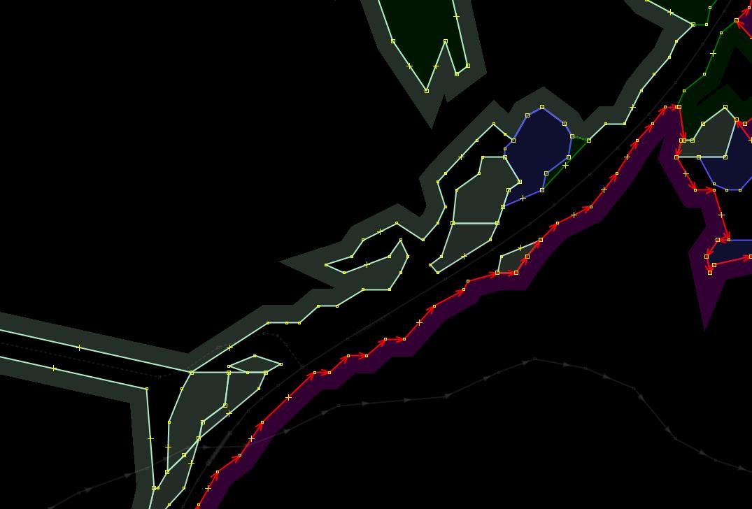
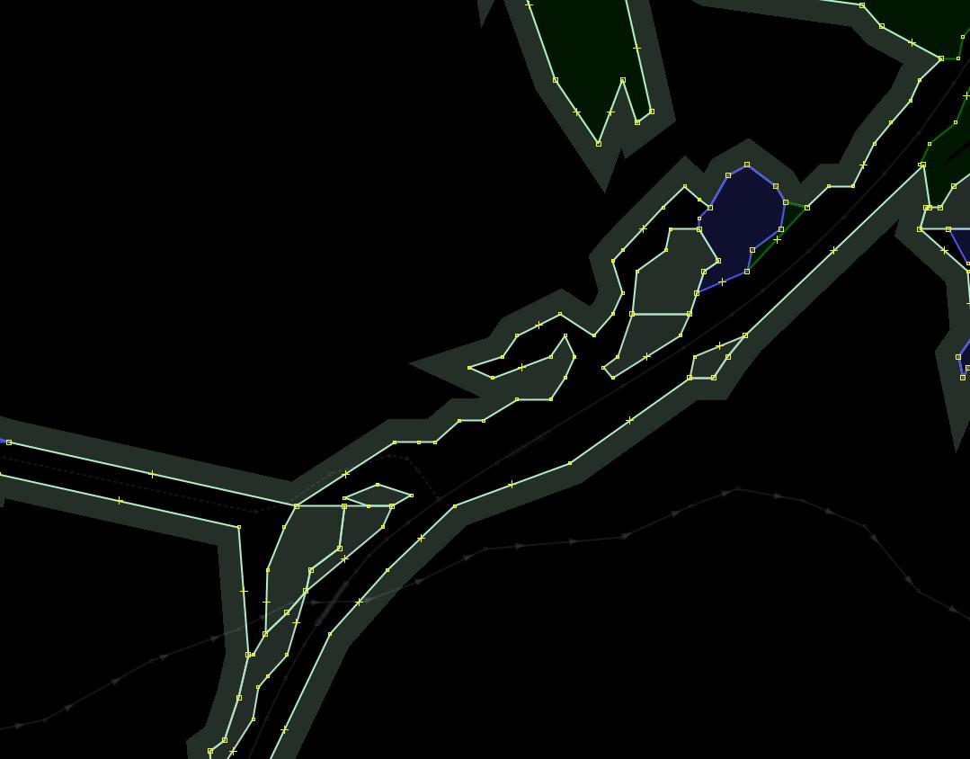
When a road goes through a forest or a field, there are often situations when a single or a small group of nodes belong to both fields, connecting them briefly, like a waistline or an isthmus, if you will. Ideally, the road should either lie completely outside any field, lie completely on top of a single uninterrupted field, or be a part of a border between these fields. See selected nodes on two examples below.

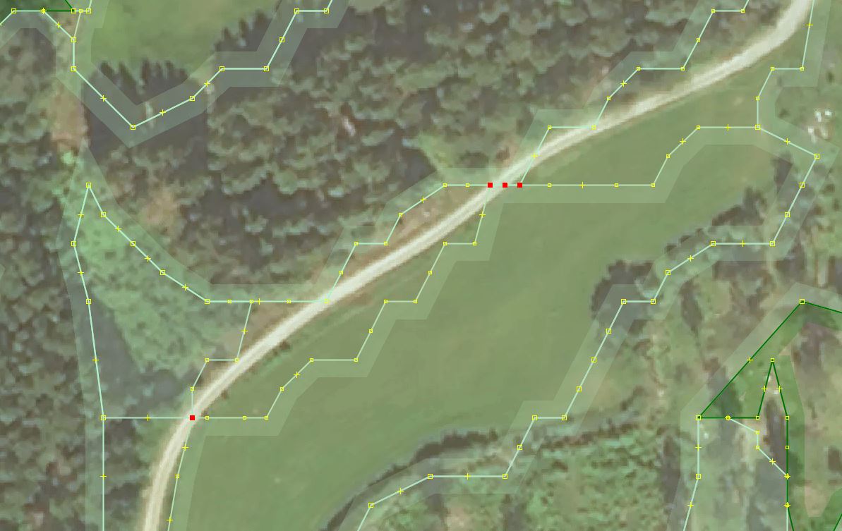
Basically there should be either three “parallel” lines (two field borders and a road between them), one line (being both a border and a road at the same time), or just one road on top of a monolithic field.

A manual solution can consist of:

• Delete the connecting node or node group placed close to the road
• Delete/fill in the empty space under the road, possibly merging land use areas it was separating
• Merge two boundaries to a single way that is also a road.

An automatic solution would be to have a plugin or data processing phase that uses existing ways for roads to cut imported polygons into smaller pieces placed on different sides of that road. Then smaller ways are thrown away as artifacts.

Current script plow-roads.py [9] mimics attempt to do something similar to this by simply removing land cover nodes that happen to lie too close to any road segment. This do ensure that isthmuses get deleted in many cases. A disadvantage is that often “innocent” nodes that simply were too close to a road get deleted, creating several types of other problems, such as too big gaps between the road and the field, too straight lines for a field border, self-intersections or even unclosed ways.

Noisy details in residential areas

There is no problem with regions already circled by landuse=residential as they go to the mask layer and efficiently prohibit any overlapping with new landcover data to be imported. However, it is not mandatory to outline each and every settlement with this tag. Often only individual houses are outlined. Besides, there are many places where even no houses are mapped yet.

Previously unmapped areas of small farms, residential areas and similar areas with closely placed man-made features receive a lot of small polygons that are trying to fill in all empty spaces between buildings, map individual trees etc.

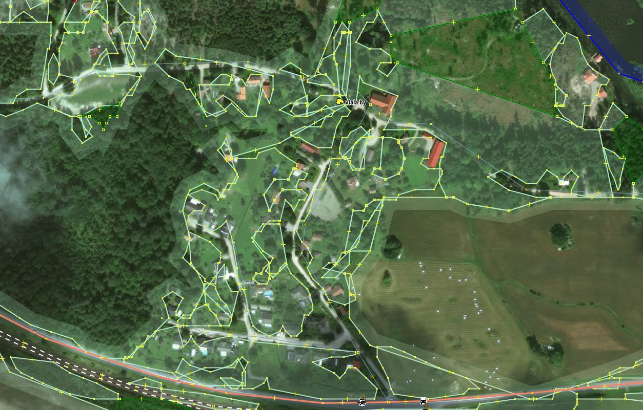
A manual solution is to delete all new polygons covering the area, as they are not of high value for man-made features. It is worth noticing that in most cases it is “grass” polygons with small individual areas. Selecting with a filter or search functions and then inspecting or deleting all ways tagged “grass” that are smaller than a certain area could speed up manual work.

However, it is hard to find all such places, leading to untidy results reported by others [5] [6].

A semi-automatic assistance method would be to buffer [13] already mapped buildings in the mask layer with about 10-20 meters distance to make sure that they are not being overlapped with landcover data. This does not solve the problem of unmapped buildings however.

Risk of editing unrelated existing polygons

Because the OSM data contains a mixture of everything in a single layer, it is very easy to accidentally touch existing features that are not part of the import intent.

Generally, for the land cover import, one is foremost interested in seeing and interacting with features tagged with landuse, natural, water or similar. Certain linear objects, such as highway and power, are also important to work on as they in fact often interact with the land cover polygons.

What is almost never important is all sorts of administrative borders. Examples of such areas are: leisure=nature_reserve, landuse=military, boundary=administrative etc. They rarely correlate with the terrain. One does not want to accidentally move them as their position is dictated by human agreements, laws, political situation etc. but not the actual state of the land.

It is recommended to create a filter in JOSM [12] that inactivates all undesirable features, still keeping them as vaguely visible in the background. This way, it becomes impossible to accidentally select them and thus change them.

Interaction with CORINE Land Cover data 2006

In general, the priority was always given to existing features, even if it was apparent that they provide a lower resolution or even notably worse information about the actual matter of things. This meant that boundaries of new features were typically adjusted to run along or reuse boundaries of old features.

In several cases when correspondence to reality was especially bad, existing features were edited to make sure their borders were in better shape. When it was possible not to have a common border between old and new features, the old ones were left untouched.

As an exception, the CORINE Land Cover 2006 [7] polygons from earlier OSM imports were not always preserved. For example, in mountainous regions they were completely replaced by the new data. They have not been included into the mask layer.

In regions with less altitude the CLC2006 features were mostly added for forests. There they were mostly preserved, at least their tagging part. However, low precision of such polygons forced to edit their borders on many occasions, adjusting nodes, adding nodes, removing nodes or rarely removing the whole feature and replacing it from the import data and/or manually redrawn data.

Removal of small excessive details

These were numerous. Typically the focus was on simplifying excessively detailed or noisy polygons generated by the scripts.

Examples of manual processing include:

• Removal of small polygons of 12 nodes and less. This was only used for certain tiles where “slivers” of polygons filled “no man’s land” between already mapped land cover polygons with double borders.

• Smoothing of polygons that follow long roads. It is typically expected that land cover borders adjacent to roads run more or less along them without any jerking unless there is a reason for it.

Because of that, the following fragment needed some manual editing:

It starts looking much more “human” after a great deal of just added nodes have been removed:

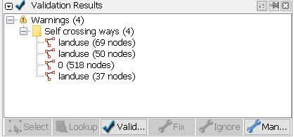
Validate, validate, validate

To validate data after major editing steps and directly before uploading means that one would run the validation steps a dozen times per a tile at least.

The base layer often gives quite a few unrelated warnings for issues that were present even before you have touched the tile.

The most common ways to fix discovered issues are to delete nodes, merge nodes, snap nodes to a line, or move nodes a bit.

The most common problems that were present in an unmodified open tile import vector layer were:

“Overlapping identical landuses”, “Overlapping identical natural areas” etc. As planned, this happened along borders of new and old objects.

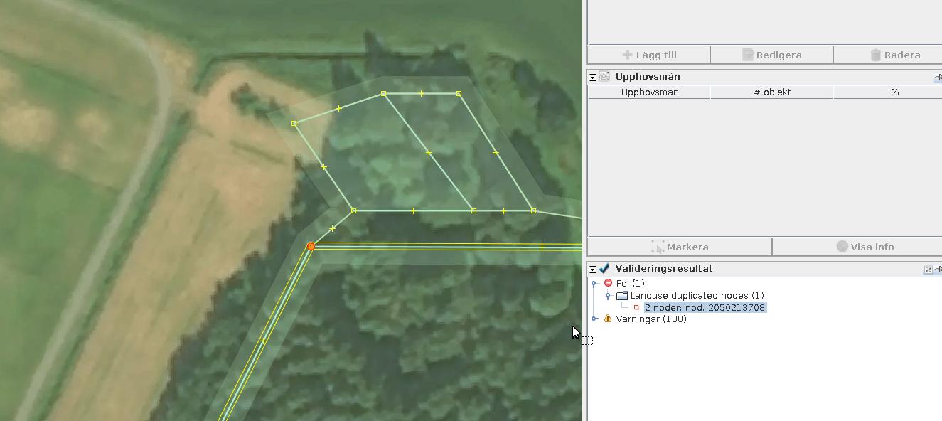
Duplicate nodes

It is easy to fix them manually by pressing a button in the validator panel.

Unconnected nodes without tags

Typically those are remnants of filtering, snapping or similar actions. If it was you who added them, these nodes can be safely deleted by the validator itself.

In the base layer, take a minute to check that any untagged orphan nodes are indeed old (more than several months old). Freshly added nodes may in fact be a part of a big upload someone else is doing right now. Because of OSM’s specifics, new nodes are added first but ways start connecting them only after later parts of the same changeset has been uploaded. The window between these two events may be as big as several hours. So do not clean up untagged nodes added by others if they were added just recently.

If you see a lone node added three years ago, then it is most definitely can be safely removed — someone else has forgotten to use that node a long time ago.

Overlapping landuse of different types, e.g. water and forest.

A small new feature that is likely to be a “sliver” of land cover squeezed between old and new data. Those can be safely removed:

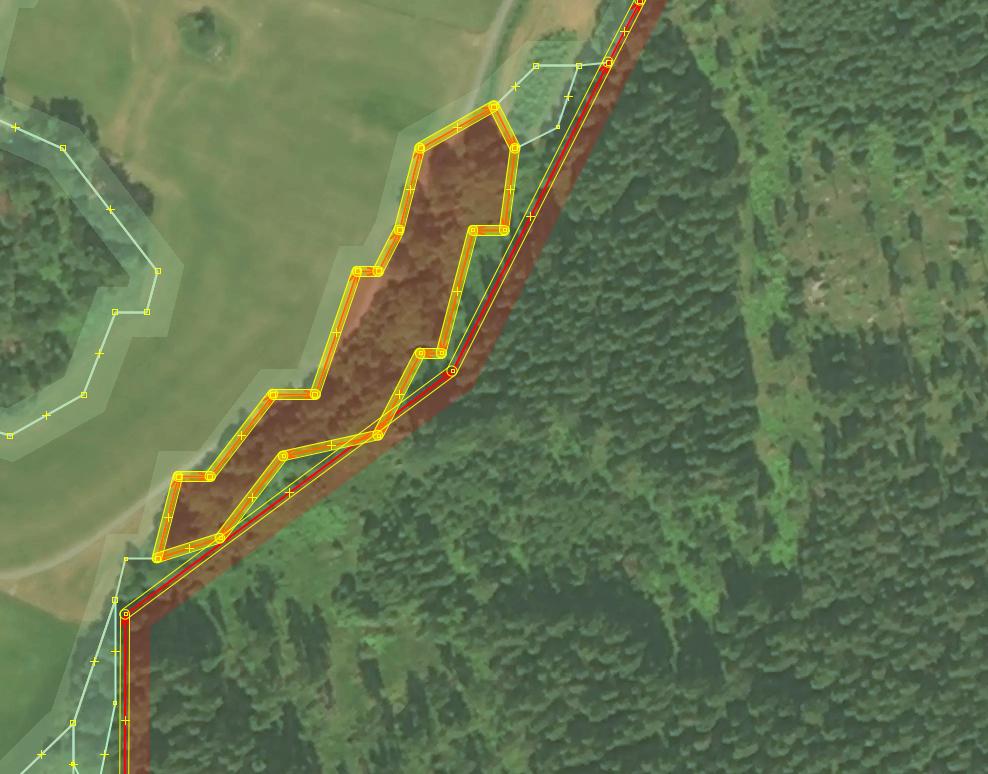
Larger new features would require creating a single shared border with an old existing feature they overlap with.

An example before:

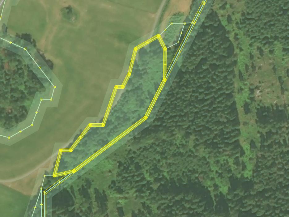
The same border after it has been unified:

Often it is possible (and reasonable) to merge two identically tagged overlapping polygons into one. Press “Shift-J” in JOSM to achieve that. This may turn out to be easier than trying to create a common border between them.

Before:

After:

Unclosed multipolygons

This was a rather awkward manifestation of a bug in plow-roads.py. Specifically, when a node connecting two outer ways of a long outer multipolygon line was chosen to be deleted, the script did not re-close the new resulting multi-way.

It did close regular ways if their start/end nodes were removed, but for the script did not track what the start/end node for more complex situations were.

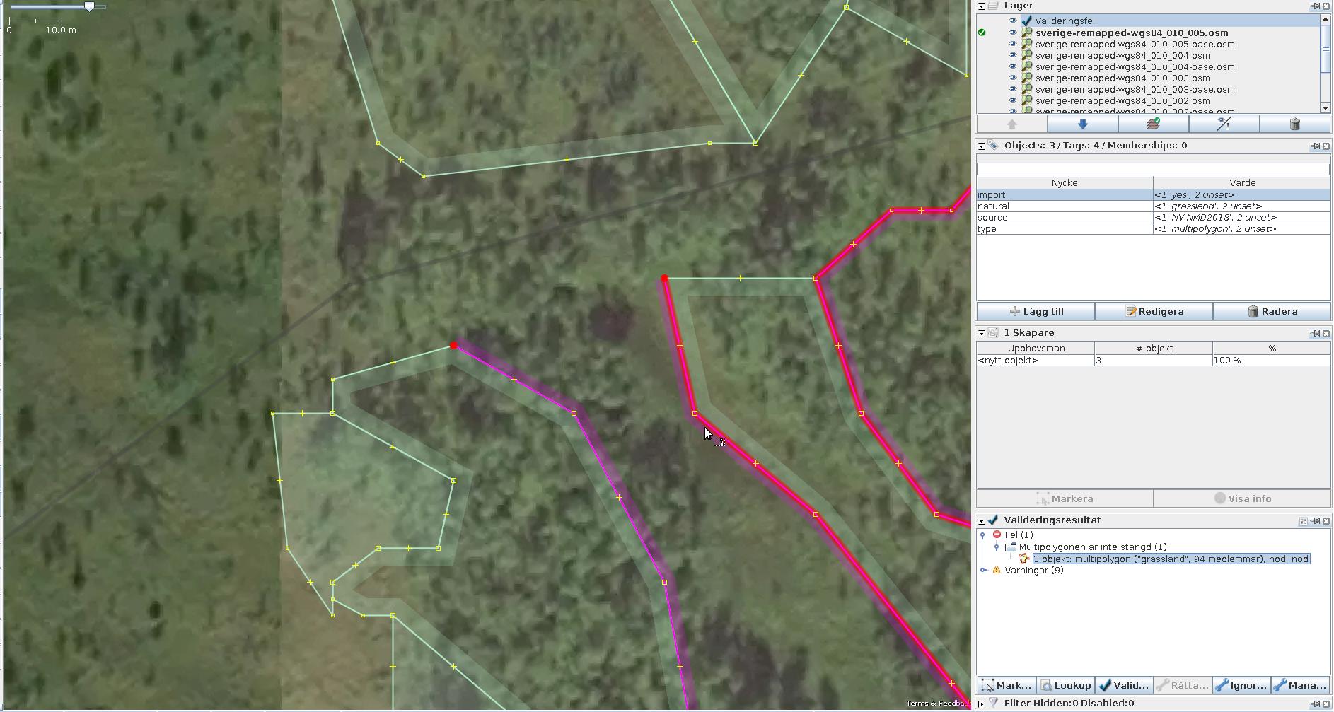
Luckily, there were not many of such situations, and JOSM validator could always detect them. And it was always trivially easy to manually restore the broken geometry by reconnecting the ways.

New islets in lakes

Islets should be marked as inner ways in lakes typed as multipolygons. However, as this import was specifically not about water objects, it was decided to left such new islets as simple polygons floating in the water. This saved time on editing lakes, many of which were not multipolygons. Their transformation from a single way into a relation can be done in a separate step.

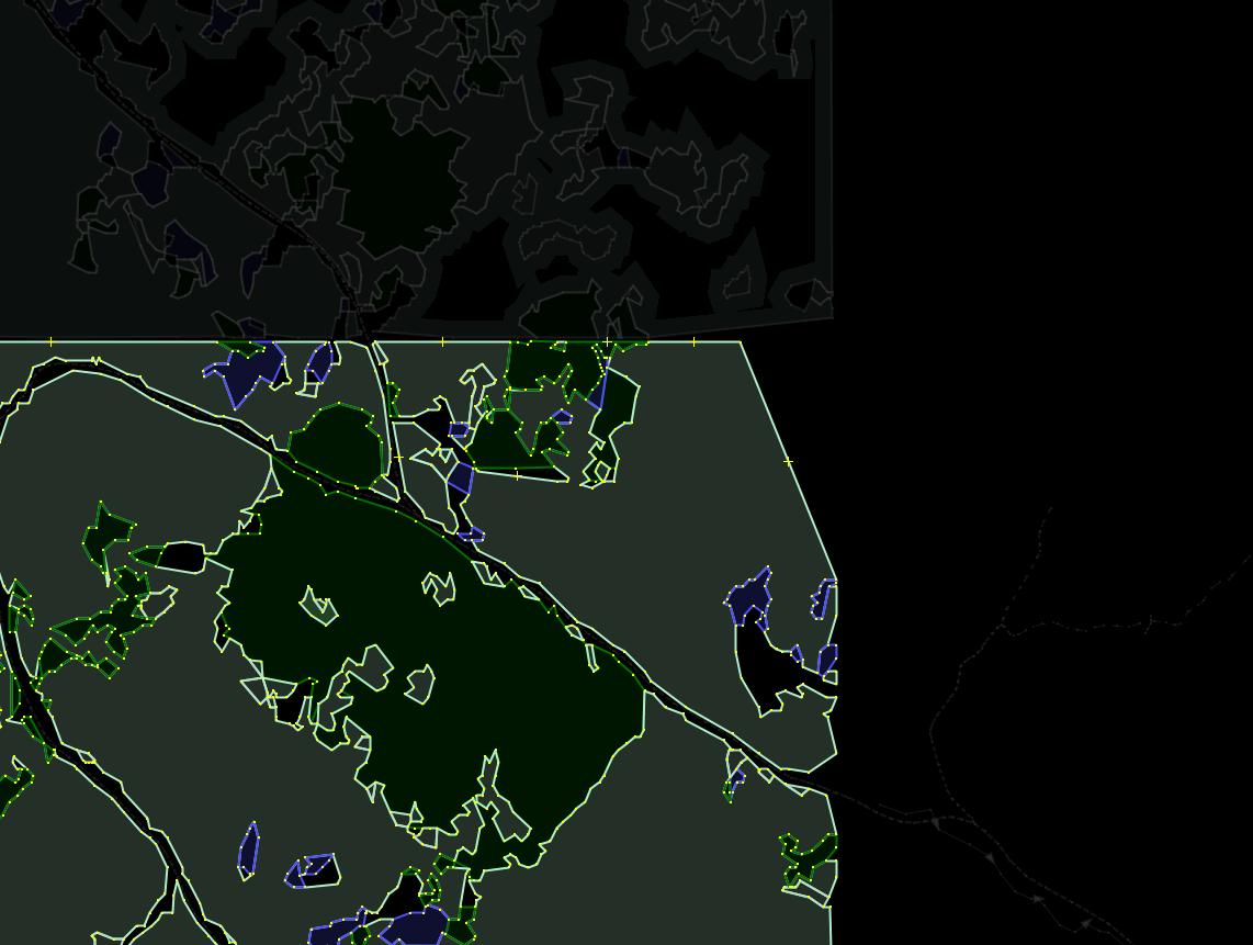
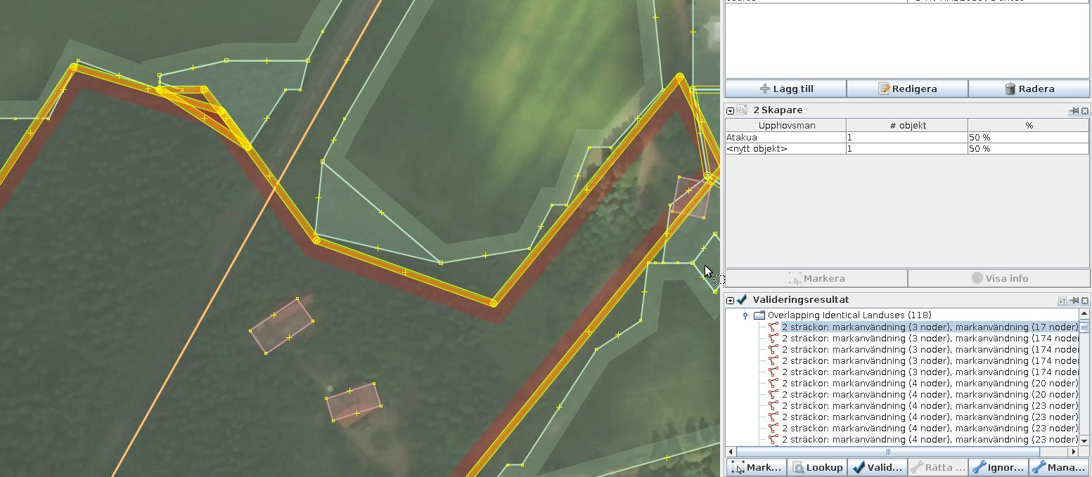
Finding an overlapping object

The JOSM validator allows you to focus on the position of most warnings. This allows addressing them efficiently. This is very efficient for cases when a bounding box for the problem is small. And this is not always then case.

It is sometimes hard to figure out how and where exactly an intersection between two polygons happens.

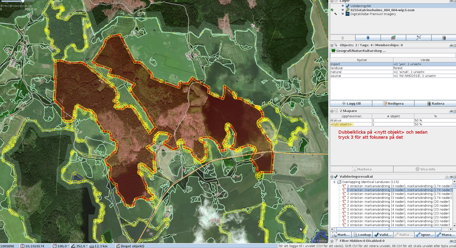
On the picture there is one huge way and several small ways which overlap with the former. It’s close to impossible to figure out individual intersections.

However, in the warnings page you can select a pair of conflicting polygons by their warning entry. And then you can select one of them (preferable the smallest one) by clicking on it, and then zoom to it by pressing 3 on your keyboard (“View — Zoom to Selection”).

Data uploading

The uploading of the resulting data starts just as a regular JOSM upload dialog. Follow the general guidelines [10].

You are very likely to have more than a 1000 of objects to add/modify/delete which will cause the upload to the split into smaller chunks. You are also likely to exceed the hard limit of 10000 objects per a changeset, meaning your modifications will end up in separately numbered changesets. None of this matters in practice as there is neither atomicity nor even ability to transparently rollback failed transactions in the project. All open changesets are immediately visible to others. You cannot easily control the order in which new data will be packed into the changesets either, so most likely your initial changesets will contain only new untagged nodes; the following upp changesets will add ways and relations between them.

Problems during the upload

For huge OSM uploads there is always risk that something goes wrong. Do not panic, everything is solvable, and this is the way huge distributed systems operate in any way.

Here are some of the problems that happened to me.

• A conflict with data on the server. This is reported to you through a conflict resolution dialog. Just use your common sense by choosing which yours and which theirs changes will stay. It is often the case that “they” means “you” as well, only the data you’ve uploaded earlier. I do not understand yet what are the specific cases when this happens, but it rarely does. Before resuming the uploading, re-run the validation one more time.

• A hung up uploading. Again, it is unclear why this happens, but it largely correlates with network problems between you and the server. JOSM does not issue any relevant messages into the UI or to the log, it just stays still and nothing happens. If you suspect this has happened, abort the uploading and re-initiate it again. Do not download new data in between. Sometimes your current changeset on the server becomes closed and JOSM reports that to you. In this case, open a new one and continue. There is nothing you can do about it in any case, so why even bother reporting this to the user?

• JOSM or your whole computer crashes and reboots. You’ve saved your data file before starting the upload, right? Open that file and continue.

If any of such problems have happened during the uploading, after you are done with pushing your changes through do a paranoid check. Download the same region again (as a new layer) and validate it. It could have happened that multiple nodes or ways with identical positions have been added to the database. In this case, use the validator buttons to automatically resolve this and then upload the correcting changeset as the last step. It is typically not needed, but to check that no extra thousands of objects are present is a right thing to do.

It is possible to “roll back” your complete changeset in JOSM by committing a new changeset [11], but it is usually not needed unless your original upload was a complete mistake.

Links

1. https://grass.osgeo.org/grass77/manuals/v.generalize.html
2. https://josm.openstreetmap.de/wiki/Help/Action/SimplifyWay
3. https://wiki.openstreetmap.org/wiki/JOSM/Plugins/ContourMerge
4. https://github.com/grigory-rechistov/snapnewnodes
5. https://lists.openstreetmap.org/pipermail/talk-se/2019-May/003673.html
6. http://grillo.users.openstreetmap.se/b353786731daa0679d8bed94907e465b2ce70029.jpg
7. https://wiki.openstreetmap.org/wiki/WikiProject_Corine_Land_Cover
8. https://wiki.openstreetmap.org/wiki/Import/Catalogue/NMD_2018_Import_Plan
9. https://github.com/grigory-rechistov/nmd-osm-tools/blob/master/plow-roads.py
10. https://josm.openstreetmap.de/wiki/Help/Action/Upload#Runningaverylargeupload
11. https://wiki.openstreetmap.org/wiki/JOSM/Plugins/Reverter
12. https://josm.openstreetmap.de/wiki/Help/Dialog/Filter
13. https://grass.osgeo.org/grass76/manuals/v.buffer.html

Written by Grigory Rechistov in Uncategorized on 26.06.2019. Tags: osm, landuse, landcover, conflation,