Atakua's Diary

Postmortem of Naturvårdsverkets dataimport to Openstreetmap

Around March 2019 I started work to import a large chunk of open data into Openstreetmap. Specifically, to improve the landcover coverage of Sweden. Mostly it concerned areas and features of forest, farmland, wetland, and highland marshes.

This post continues and somewhat concludes the series of thoughts I’ve documented earlier in 2019:

The import plan documents a lot of technical details. I maintained it to reflect the high level overview of the project throughout its life.

Why bother

My motivation behind the project was that I was tired to trace forests by hand. My understanding is that it would take a million of hours to finish this work by using manual labor alone. I, being lazy, always look for ways to automate it and/or integrate someone else’s already finished work.

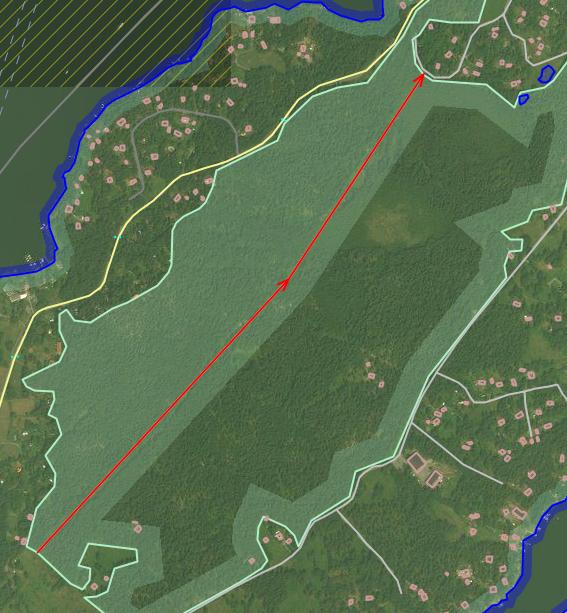
And there is a lot of work to integrate. Here’s how the map looked like before the start of the project:

Overview of Sweden's unmapped land cover for start of 2019

There is other peoples’ work worth integrating. Many national agencies around the world now offer the geographical data they have collected and continue to maintain to everyone under liberal licenses, such as CC0 or public domain. To me, it looks strange to not even to attempt make use of this data.

Note on terminology

I will use “land cover” and “land use” as synonyms, even though they are not. But I do not care enough to make such a difference, and nobody else seems to do it as well de-facto, given the current tagging status. People predominantly use “landuse=*”, “natural=*” and “residential=*’ tags to convey details both for land use and land cover. At the same time, almost non-existing presence (and lack of support by renderers) for “landcover=*” makes it questionable to add this tag for new data. Nobody will see the results of such work.

The main idea of the import

Naturvårdsverket’s land cover dataset comprises of a single (huge) GeoTIFF where every 10×10 square meters of Sweden’s surface is classified to be one of predetermined types of land cover: forest, water, roads, settlements etc. So it is raster data, while Openstreetmap uses vector features, such as polygons and multipolygons, to represent land cover. So the first step would apparently be to convert raster to vector. Resulting vector will certainly have discretization noise (“90-degree ladders”), so the next required step is to smooth vector to look more natural.

To make sure newly added polygons do not conflict with already present map features, it was required to merge two vector datasets, or to conflate them. Need for conflation meant that some parts of new vector data had to be adjusted. Among these modifications were: delete whole polygons, cut polygons, align borders of new and old polygons, retag certain pieces to change their tags, and so on.

Because the input dataset is really huge, it would be unreasonable to attempt importing it in a single pass. Thus, I needed a strategy to split input data into chunks. This meant that new, artificial boundaries would start to appear inside the vector dataset. As it will be shown below, such artificial boundaries adds certain unique challenges to the process.

Openstreetmap’s uniquely loose data classification scheme makes it impossible to algorithmically decide on whether any new data would be well enough integrated without duplicating or unnecessarily overlapping anything already existing on the map. Thus, the final step for each data chunk before it gets uploaded was to visually inspect the result of merging of two layers and to fix uncovered problems.

Evolution of the process

There have been several iterations, some of them huge, requiring regeneration of everything from the start, some were regarded as smaller touch-ups. I can now recall several major decisions that affected the result in a significant way.

Import one kommun at a time. This was the original plan to have 290 disjoint chunks made, then edited/uploaded to the OSM. Quite a few of vector OSM files turned out to be larger than 1 GByte of XML. However, the division of the territory into kommuns remained in some form through the rest of the project.
Be less aggressive with smoothing. As the Vingåker experiment (see below) demonstrated, it was necessary to try several values of thresholds and several available smoothing algorithms to find something that does not destroy too much of polygons but removes excessive details.
Cut kommuns into smaller “rectangular” tile 0.1×0.1 degrees latitude/longitude. Each tile then could be loaded into JOSM without much consuming all the RAM. It still could contain tens of thousands of nodes and usually required several changesets to upload everything. Because of the significant overhead of manual re-sewing of tiles (see below), I considered increasing their dimensions to be 0.2×0.2, but never did it.
Pay special attention that adjacent tiles do not overlap. It was discovered during Katrineholms kommun import that coordinate system transformation performed too late resulted in overlap between adjacent tiles (by up to hundres of meters). To prevent it, it was made certain that data gets converted from SWEREF99 coordinate system to WGS84 (the one used by OSM) early at raster stage.
Employ a second, “negative” raster layer produced from existing OSM land cover data. Its purpose is to to mask data points in the import raster data as if nothing was known about them. My original intersection detection heuristic only considered bounding boxes of polygons. Being too imprecise, it generated excessive amount of false positive matches, causing a lot of perfectly good new polygons to become rejected at conflation. By masking new raster data with “old” rasterized data meant that traced vector polygons could not possibly overlap with old ones (except inside a thin “coastline” buffer zone caused by the discretization noise). Of course, using two input raster images required to regenerate all the vector data from scratch.
Add buffered roads to the negative layer. After some consideration it was decided to include existing OSM roads to the negative raster layer. Their position correlated with “road” land cover pixels in the input raster data, and excluding areas around them allowed to have less noise in the result. “Roads” include railroads, motorways of all sizes and also pedestrian ways down to trails. Inclusion of trails (highway=path) turned out to be a questionable decision.
Add water to the import. Originally I expected even smallest lakes to be already well-mapped in OSM, and therefore did not include water-related polygons, such as lakes and even wetland. However, visual inspection of conflation results uncovered that the situation was much worse than I thought. Even quite large wetlands were missing. Late in the project I decided to retain information about water and to convert it into “natural=water” and “natural=wetland” polygons. It also had to use a modified conflation specific to monolithic areas (see below).

Besides these bigger changes, throughout the project I constantly adjusted a multitude of numerical parameters affecting the conversion process, such as cut-out thresholds, smoothing parameters, and so on. Used algorithms and tools have also received numerous fixes and adjustments.

Tools used and made

Of course, the JOSM editor was the main and final tool to process data before uploading. Some adjustments to Java VM memory limits were needed for it to be able to chew through larger chunks of the import. Having a machine with 32 GB RAM also helped.

I initially used QGIS to visualize input data and iteratively apply different hypothesis to it. However, this application turned out to be not very amenable for scripting. After some time struggling with it, I realized that I essentially used QGIS as a front end to another GIS called GRASS. I ended up using a multitude of GRASS’ individual instruments such as v.generalize, v.clean etc. to construct data processing pipelines taking raster data and chewing it multiple times until vector data was out.

Among libraries to process, convert and otherwise transform data, GDAL was of utmost value to me, both directly and indirectly via all GRASS tools based on it.

Besides many existing tools and frameworks , I’ve written quite a few lines of Python, Java and Bash scripts to assist with data conversion, filtering, cleanup and conflation. Currently the bulk of this code is at Github and my other repositories, and I continue to reuse some pieces of it for my ongoing projects.

Results

The project resulted in things both visible to others in a form of the map improvements, and also as a lot of knowledge for me and hopefully for others.

What required no improvements

Of all the kommuns quite a few have already been mapped well enough. Adding new data for them would mostly imply a lost of manual cleanup work without significant improvements for the coverage. As expected from the beginning, examples of such well covered municipalities were areas around the biggest cities, such as Stockholm, Göteborg, and Malmö.

The farther to the north, the less land cover data was present in OSM, the more need for data import seemed reasonable.

What was covered by new data

Kommuns borders were selected as the top level of hierarchy to determine import structure form the beginning. However, it turned out to be impractical, as sizes of such import units varied wildly, areas of kommuns were often too big to visually review in one sitting, and geometry of borders turned out oftentimes to be too convoluted (long and twisted, with enclaves and exclaves etc.), with no practical benefits coming from from blindly obeying them.

Somewhere in the middle of the project these boundaries were only used as rough guidelines for splitting data into tiles. All tiles were of fixed size and alignment, and as such could span over the boundaries of kommuns.

The following parts of the country were completed, fully or partially.

Vingåkers kommun. It was the first one and the only one converted, conflated and committed as the whole in one go. Being the first one, a lot of mistakes were admitted together with the data, such as overly aggressive Douglas-Peucker simplification.
Katrineholms kommun. I started to manually map this area long before, then tried to employ scanaerial plugin to assist with tracing forests. Around 50% of the territory was prepared by these means. Finally I finished it with the import data. As the location was adjacent to just finished Vingåkers kommun, it was the first experience where I had to tackle the requirement to nicely align polygons for adjacent parts of the import.
Vadstena and Åstorp. Relatively small subareas which are mostly covered by farmland. Here I tuned my algorithms and learned to expect unusually tagged (multi)polygons to conflict with new data.
Linköpings kommun. It was basically the only support I received from someone else during this project. I have not participated much in working on this kommun, and the data used for it, as far as I can tell, was from one of the first batches that I have provided, and as such it included no improvements that were present in later iterations.
Åre kommun was my biggest effort so far. Result of many laborious evenings, nights and days, the kommun has been mapped in the fullest. Besides the territory of the kommun, adjacent parts of the country (e.g. parts of Bergs kommun) were also mapped. More details are in my previous post.
Ljusdals kommun. Compared to earlier work, here I started to map water areas in addition to forests, farmland and other “ground” cover. I discovered that the situation with mapping of smaller lakes in Sweden was not as good as I originally assumed. Imported water polygons included smaller lakes and medium-sized rivers and streams represented by “non-zero width”. Compared to ground cover, water polygons had to be treated as monolithic (see below), which was reflected in conflation script adjustments. However, I did not finish this kommun. All work essentially halted after that.

What was not covered and why

Remaining kommuns did not receive significant changes. While there were no technical reasons to stop at this point, I was unable to reduce amount of manual work to a level low enough to allow a single person to finish all tiles in reasonable time.

Work on Åre kommun demonstrated that individual tiles required up to 30-60 minutes of manual work each to import. This is still faster that one can trace an area of the same size with the same level of details. Manual operations that had not been optimized to be done by the scripts were becoming tedious to me though.

Fixing geometry warnings such as self-intersections. Despite all attempts to detect and address the majority of self-intersections at vector simplification phase, to have up to 100 warnings per tile reported by JOSM Validator was not uncommon. Absolute majority of them were trivial short “loops”.
Sewing tiles’ boundaries. Adjacent pixels of the source raster that happened to land inside separate adjacent raster tiles were converted to unconnected vector features. This created a tiny but non-zero gap between them. I’ve employed certain heuristic algorithms to close this gap when it was safe. Yet, almost every vector tile required to manually scroll along its border in JOSM and to sew the remaining gap between it and already uploaded adjacent tiles.
Addressing quality problems of pre-existing data. It was not uncommon to meet situations with roads traced by offset landsat imagery, crudely drawn polygons for lakes and forests etc. Given that this OSM data was also used for generation of the negative raster layer, these problems could also be imprinted into the new vector features to be imported.
Merging boundaries of new and old polygons. Ideally, this should have been the only type of manual work needed for each tile. In reality, this was a relatively smaller part of the manual work.

I go deeper into technical details behind some of these problems below.

Problems

It’s time to complain. A few factors were discovered along the way which I tend to classify as external problems, common for any other sort of future importing work attempted for the OSM project.

The OSM community’s inconsistency towards imports in general and land cover imports in particular. Not many of arguments DH4 or higher was given to me. I won’t delve deeper into the social, humanitarian, technical, economical, legal and political circumstances known to me leading to this situation. Let’s just say I have no desire to read or to write to the OSM Imports mailing list ever. Conversations on that mailing list, while not being openly toxic, tend to derail into delving over general unsolved/unsolvable issues of the whole project. This brings little constructive feedback to the initiator of an import effort, while forcing him/her to drown under disproportional volume of email exchange. There are deliberately no objective formal/verifiable/measurable criteria of acceptance, meaning everyone is judging data from his/her standpoint of “beauty”. There is no authority to have a final word in a discussion, and there are no procedures for voting for/against a proposal, which gives disproportional power to those few with louder voices. By the way, barely anyone has commented anything on the import plan topics. No comments on the quality assurance sub-topic, for which I was so much hopeful. It seemed that spending so much time on documenting the project was redundant.
Rounding of coordinates done on server. I was baffled to discover that, after I have thoroughly made sure that no self-intersections are present in data and have uploaded it, then to download it back and to see my polygons to self-intersect! It looked like nodes were moved a tiny bit when they were returned from the database. Comparing the original data files and copies downloaded from the OSM, I could notice that coordinates precision had been lowered. Only 7 digits after the dot were kept. At the same time, JOSM (and its tools like Validator) are perfectly capable of operating over coordinates with 10 or more digits after the dot. It seems that one needs to take this into account when running geometry checks.
Poor validation tools for multipolygons. Neither offline nor online tools, nor JOSM nor Osmose, seem to report intersection/overlapping of multipolygons. From the practical standpoint, overlapping multipolygons is the same problem as overlapping polygons. It may be technically harder to implement and computationally more costly to run such a check, yes, I do realize that. But at least some basic checks, or even imprecise algorithms (with reasonably low ratio of false positives) would still be better than nothing. I’ve spent quite some time hunting for rendering problems caused by omissions made in multipolygons (e.g. because of the implicit rounding problem).
No tools for conflation of (multi)polygons. As OSM community still manage to somehow import zero-dimensional (i.e. POIs) and linear features (i.e. road nets) from time to time, a few tools to assist with conflation of those types of features exist. However, it is not the case for import data in form of closed polygons. Most of my hand-written tools were made because nothing better (or anything really) existed for my goals. I do understand that polygons and especially multipolygons are much harder to work with than e.g. roads or POIs. This, however, does not excuse the fact that nobody has prepared tools to for merging, splitting, transforming etc. them.
Obstacles of using GIS-software to perform read-modify-write cycle over the OSM contents, especially the “write” part to preserve untouched objects in unmodified state. The rounding problem above is an example of such an issue. Loading OSM data into another GIS format and then immediately exporting it (without any explicit modifications) can still produce a dataset not identical to the original one.

Useful tricks learned

Add comments describing operations and decisions made over primitives to the primitives themselves as tags. All warnings issued by scripts should be turned into “fixme” or similar tags. Then nodes with these tags can easily be highlighted in JOSM at the visual inspection phase.
Save both “survived” and “dropped” primitives into separate files to simplify debugging and to record reasons why a certain feature was kept or deleted from the dataset.

The data flow approximately looks as follows:

new data                  review-ready data (with additional fixme tags)
         ---conflation-->
old data                  dropped data (with new note tags)

Experience to be used later

There are better tools out there

One excellent tool I’ve discovered too late was ogr2osm. GRASS GIS worked best with vector data in GML format, while JOSM understands its native OSM XML format best.

JOSM’s GeoJSON and GML support was lacking at that moment. I ended up writing my own converter from GML to OSM, but using ogr2osm is excellent for such work. I plan to use it instead in the future.

Node snapping is treacherous

There are often two vector features and they need to be adjusted to have a common segment. One may think that automatic snapping — moving/merging nodes of a source line that are close enough to the destination line — would do the job in a second. But so many things can go wrong with it.

Which nodes to snap. Only nodes closer than a pre-defined threshold should be selected for modification. The distance threshold value cannot be automatically deduced by an algorithm as it mostly depends on input data resolution, its quality etc. It often happens that the threshold has to be adjusted for different parts of the same input.
Where to snap. A single node chosen to be snapped may in fact “gravitate” to multiple destination segments, or multiple points on the same line. Let’s suppose that the chosen snapping threshold is too big, bigger than linear dimensions of the destination polygon. In such extreme situation the source node may end up glued to any position of the destination.
In which order to snap nodes. In the end, it is not individual nodes but two lines that we care about. Snapping is expected to preserve the original order of nodes on both lines. For reasons outlined above, it may not happen automatically. What can happen is erratic “jumping” from of segments. At the very least, snapping should be accompanied by a cleanup phase that detects and corrects created problems.

To quote v.clean tool=snap manual page:

The type option can have a strong influence on the result. A too large threshold and type=boundary can severely damage area topology, beyond repair.

I have some ideas about a type of iterative snapping approach. Lines are “stretchy” and “flexy” and are “attracted” towards each other. Attraction forces compete against repulsion forces. As a result a most “natural” (i.e. with minimal potential energy) relative position of lines is achieved. I however do not know how hard it would be to fine-tune parameters of the attraction/repulsion forces for the process to be stable enough, and whether performance of such an algorithm would be enough for practical use.

Keeping knowledge about sewing points is important

When splitting bigger geographical data files into smaller chunks by arbitrarily chosen (i.e. not dictated by the data itself) borders, try to keep information about split points to simplify re-gluing of adjacent resulting data. Without such information, split points should either be detected algorithmically, which is not trivial nor reliable, or specified manually, which is more time-consuming than one would think.

It does not matter whether data is organized into regularly shaped rectangular tiles, or follows less regular but nevertheless arbitrary administrative borders.

Ignoring the problem won’t help either as it would result in unconnected linear features and gaps and/or overlaps for landcover features.

Of course, the aforementioned problem does not affect zero-dimensional imports, such as POIs. They can be organized in arbitrary subsets without disturbing any sort of (non-existent) relational information.

Here are some ideas on how to handle the re-sewing problem.

Vector input

For vector polygons, maintain correspondence between unique node IDs used internally by your source (i.e. negative numbers for OSM XML files) and unique node IDs assigned to them by OSM database after they were successfully uploaded. Let’s suppose two polygons are uploaded independently as they are in different tiles. To avoid uploading duplicate nodes shared by them, after the first polygon has been uploaded, their IDs (and their refs) have to be updated in the second one. This way, corresponding points will only be uploaded once. Uploading the second polygon will refer to their already present instances instead of introducing duplicates with different IDs.

Alternatively, duplicate nodes can be merged after everything has been uploaded, as detecting them should be easy. However, this is less elegant, and creates some room for mistakes, as we essentially recreate shared borders instead of preserving them in the first place.

Raster input

For raster data, the process is more involved, as the vectorization phase and follow-up simplification passes can easily move nodes and destroy relation information close to tile borders. Recovering such information from adjacent vector polygons is even less reliable as it involves some sort of node snapping to lines. Node snapping involves moving of existing or adding new nodes and therefore it is capable to corrupt geometrical properties of polygons: create self-intersections, loops etc. I can imagine two approaches to the problem.

Modify vectorization algorithms to treat tile border pixels and nodes produced from them in a special way. Resulting vector features should retain information about which segments were traced from tile boundaries. The same applies to line simplification algorithms: they should not move nor delete nodes originating from tile borders.
Use natural borders present in the data to determine form and boundaries of smaller chunks. For example, if exclusively tracing forest areas, linear borders, such as water coast lines, (buffered) roads, rivers etc. can be used to delineate where a free-form chunk ends. The problem with this approach is that there is no guarantee about result’s size, form or run time. Basically, a single stretch of forest can span through the whole country. Inevitably, artificial cuts have to be introduced into the data. To minimize their length while keeping the size of chunk within limits would be an interesting challenge.

It is not only me who considers tiles borders to be an issue for automatic processing of geometrical features. From Facebook’s RapiD FAQ:

Why does RapiD crop roads at task boundaries? Are you concerned about the risk of creating disconnected ways?

We believe this is a general problem when working on tiled mapping tasks. We learnt from the community that when working on tasks on HOT Tasking Manager, a general guideline for the mappers is to draw roads up to the task boundary to avoid creating dupes across tasks, so RapiD is designed to align with this guideline. When the user is working on the neighbor task later, the close-node check or crossing-way check will have a chance to catch the disconnected ways and help the user fix them.

So far, I used the “natural” borders approach in a limited form. Roads running through forests cut them into smaller bits. For rectangular tile borders, a lot of manual work was needed to recover common borders late into the process, because the vectorization and simplification tools I used did not care about preserving required information.

Monolithic and non-monolithic features

Here is another concept I’ve discovered when I’ve decided to import water polygons.

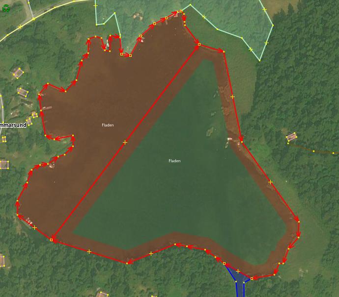
For forest areas it is quite OK to split them along arbitrary borders. Generally, someone who maps forest areas manually starts by drawing its border until he/she becomes tired or hits the limitation of max 2000 nodes per way. Then current portion of forest gets closed with random long straight lines going right through the forest mass so that the polygon become closed. This polygon then gets uploaded. The next adjacent section of the same forest is then traced the same way, combining “real” borders and the previously drawn artificial border. The picture below illustrates this situation.

Non-monolithic forest

However, closed water objects, such as lakes, even huge ones with borders spanning well over 2000 nodes (and thus represented as multipolygons), are traced and treated differently. People do not tend to create arbitrary internal borders for them.

In other words, there are few examples when a lake gets treated like this:

Non-monolithic lake

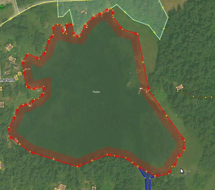
Instead, a nice single polygon is usually drawn:

Monolithic forest

It seems that land cover classes, among other classes of area-like features, can gravitate to one of the following types.

Non-monolithic land cover for which arbitrary internal borders are allowed and are in fact welcomed to maintain feature size in check. Examples are: forests, farmland, long riverbanks.
Monolithic land cover, where feature size does not justify splitting it into arbitrary delineated chunks. Lakes are most prominent examples, even such complexly shaped as Mälaren. A feature with defined name have more chances to be treated as monolithic. When there is a single name, a single feature seems reasonable. But it gets impractical for e.g. riverbanks which may be very long.
Land cover with undefined traditions or rules. An example would be wetland. I would risk to say that wetlands are even more mysterious for average mappers (such as myself) than forests. There are so many types of them, their borders are even less defined than forests’. Sometimes it makes sense to treat them as more water-like type, other times it is convenient to consider them have forest-like behavior.

Import raster data already has arbitrarily defined split lines. These lines may split monolithic features into two or more vector pieces. This is undesirable as this goes against the tradition of mapping such features.

For this reason it was decided to pay special attention to new water polygons lying close to tiles’ borders and, when needed, to merge multiple pieces back into a single object. This, however, had to be done manually.

A good thing with monolithic features however is their “all or nothing” nature, which can be used when conflating them against already mapped counterparts. A special algorithm compared “closeness” ratio of borders of an new and an old water features to decide whether or not they corresponded to the same object. Such comparison would make no sense for non-monolithic features as they may have parts of borders arbitrarily defined by a user’s will, not by properties of the physical world.

Additional results

My better understanding of Openstreetmap’s intrinsic conflicts and different views, including sorts of idealistic philosophy some people preach. Anarchy allowed in certain aspects of the project existence clashes against the desire for rigid control in other aspects.
Tools for operating over OSM files and related vector formats, available at Github. They surely duplicate a lot of functionality already existing in GIS-systems. Surely these tools are mostly useless for anyone but myself because…
There are much better programming tools available for processing geometrical information. And I need to learn these tools and to start using them. Libraries such as shapely, ogr, (geo)pandas and others exist and they could have simplified some of my work if I knew about their existence in advance. Osmosis is an OSM-focused framework I might also need to learn a bit.